I finally got around to hardcore studying motor theory this winter break, and decided to write (partly as an exercise, but mostly because I think it’ll be a helpful tool) a python package for running transient motor simulations. The idea is that with a couple lines of code, you can simulate the performance of a “typical” salient or nonsalient motor combined with an arbitrary control algorithm and get useful data for either tuning or designing a motor controller. For example, for a motor with more than one pole pair, an inverter driving a three-phase set of sinusoids that’s unsynchronized generates less torque than a control type that just focuses on synchronization:

The difference is pretty clear. This is something that I was initially confused about early on in making motor controllers, but if I had this back then, the problem would’ve been obvious!

Most of the simulation outputs here are with made up numbers so that the units are more pleasant to look at.

Nonsalient Motors

Simulating nonsalient motors (where $L_{d} \approx L_{q} $ is pretty straightforward. You should read Ben Katz’s notes on this. Here, they are simulated the same way using RK45. “Plugging in an inverter” really just means that the command voltages $ V $ are set based on the controller output during the update step. Torque is computed using the definition in the dq frame: $ \tau = \frac{3}{2}N_{pp}\lambda_{PM}i_{q} $, only because I find this definition more intuitive.

The simulator can also simulate switching effects. Aside from being kinda cool to look at, this is important because the switching effects increase total harmonic distortion, which decreases power factor. This is important because it contributes to loss, but also increases stress on reactive components in the inverter, like DC link capacitors. I’ll get to this later.

Salient Motors

Although most BLDCs are nonsalient¹, since I’m working on a traction inverter for Motorsports and we’re using IPMs (which are salient), I’m including them. Saliency is defined in the dq frame, so it makes sense to simulate there too. The RK45 update step transforms the commanded per-phase voltages to the dq frame, computes the torque output and returns $\frac{di}{dt}$ for the next iteration. The core equation, in matrix form, is just the dq voltage equations:

\[\begin{align} \frac{d}{dt} \begin{pmatrix} i_{q} \\ i_{d} \end{pmatrix}=\begin{pmatrix} L_{q} & \\ & L_{d} \end{pmatrix}^{-1}(\begin{pmatrix} v_{q} \\ v_{d} \end{pmatrix}-\begin{pmatrix} R & \\ & R \end{pmatrix} \vec{i}-\omega_{e}( \begin{pmatrix} & L_{d} \\ -L_{q} & \end{pmatrix} \begin{pmatrix} i_{q} \\ i_{d} \end{pmatrix}+\begin{pmatrix} \Psi_{R} \\ 0 \end{pmatrix}) \end{align}\]

Obviously, inverter current limits weren’t simulated there.

Optimization

Saliency introduces a reluctance torque term $ \tau=\frac{3}{2}(L_{d}-L_{q})i_{d}i_{q} $ in the motor equation that makes the torque dependent on both the d and q axis currents:

\[\tau=\frac{3}{2}(N_{pp}\Psi_{R}i_{q}+(L_{d}-L_{q})i_{d}i_{q})\]

This makes it unclear how to maximize torque generation, especially at higher speeds, where backemf gets close to the bus voltage and the balance between $i_{d}$ (field weakening for more possible current output) and $i_{q}$ (more permanent magnet torque) needs to be met. It turns out that optimizing this isn’t that difficult. First, consider maximizing the torque for a given speed; this should give the torque-speed curve of the motor. Torque increases with currents, so there clearly needs to be a current limit, which is just given by the per-phase max current output of the inverter (typically determined by switch limits). Since the optimization is in the dq frame, this per-phase limit needs to be transformed first to the $\alpha \beta$ frame (for delta and wye termination, this is related by a factor of $\sqrt{3}$ ), and can then be set with a magnitude limit:

\[i_{\alpha}^2+i_{\beta}^2 = i_{d}^2+i_{q}^2 \leq \frac{I_{ph(max)}^2}{3}\]

At low speeds, when the backemf is still low, the torque speed curve is current limited, but at high speeds, it’s voltage limited. The voltage limit, much like the current limit, just requires a transform from the per-phase constraint to the $\alpha \beta$ frame, where the vector magnitude allows relating the constraint to the dq frame:

\[v_{\alpha}^2+v_{\beta}^2 = v_{d}^2+v_{q}^2 \leq \frac{V_{ph(max)}^2}{3}\]

$v_{d}, v_{q}$ are defined as a function of the d/q axis currents and backemf terms. Unfortunately, they’re also a function of $\frac{d}{dt}i_{dq}$, which makes optimization inconvenient, but this can easily be solved by only considering steady state:

\[\begin{align} v_{d}= Ri_{d}+L_{d} \frac{d}{dt}i_{d}-\omega L_{q}i_{q} \\ \to Ri_{d}-\omega L_{q}i_{q} \\ v_{q}=Ri_{q}+L_{q} \frac{d}{dt}i_{q}+\omega(L_{d}i_{d}+\Psi_{R})\\ \to Ri_{q}+\omega(L_{d}i_{d}+\Psi_{R}) \end{align}\]

And now the optimization can be fully defined:

\[\begin{aligned} & \text{Minimize:} & & \tau=-\frac{3}{2}(\Psi_{R}i_{q}+(L_{d}-L_{q})i_{d}i_{q})\\ & \text{Subject to:} & & \left\{ \begin{aligned} v_{d}^2+v_{q}^2 \leq \frac{V_{ph(max)}^2}{3}\\ i_{d}^2+i_{q}^2 \leq \frac{I_{ph(max)}^2}{3} \end{aligned} \right. \\ & \text{Where:} & & \left\{ \begin{aligned} v_{d}&=Ri_{d}-\omega L_{q}i_{q} \\ v_{q}&=Ri_{q}+\omega(L_{d}i_{d}+\Psi_{R}) \end{aligned} \right. \end{aligned}\]

Sweeping over a variety of speeds gives the maximum torque at that speed as well as the proper d/q axis currents to hit that operating point while considering field weakening effects. Notice that field weakening isn’t a special case here!

Here’s the torque-speed and power-speed curves from the datasheet of the AMK motors we’re using for motorsports:

And here is the simulated one, using values from the datasheet as motor parameters and a bus voltage of 500V (matches the orange “+field weakening” plot):

The simulated one is pretty close, and I think the only meaningful difference is random losses at higher speeds (friction and core loss mainly, I think).

For torque vectoring though, you want to be able to command a specific torque, not necessarily the maximum, for a given speed. That makes the torque the constraint, and since the most typical operating region of the motor is in the current constrained region, it makes sense to make that the objective function:

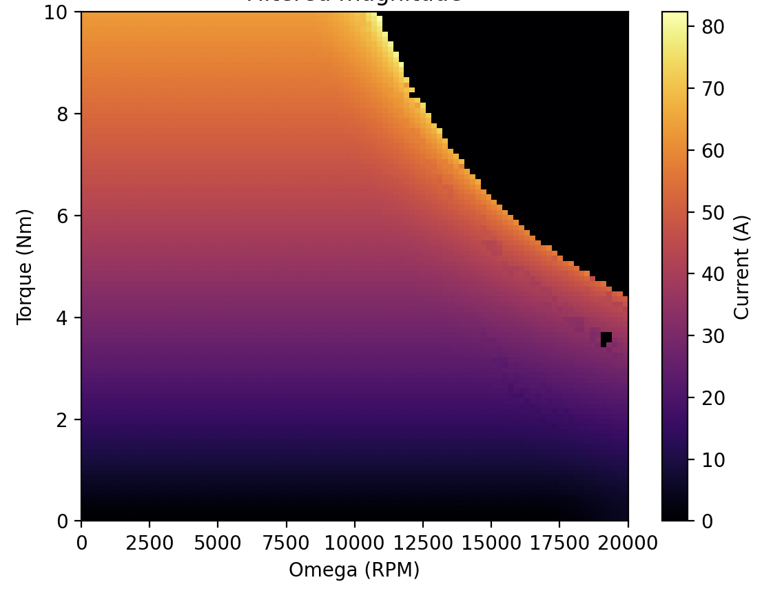
\[\begin{aligned} & \text{Minimize:} & & i_{d}^2+i_{q}^2 \\ & \text{Subject to:} & & \left\{ \begin{aligned} \tau=\frac{3}{2}(\Psi_{R}i_{q}+(L_{d}-L_{q})i_{d}i_{q})\\ v_{d}^2+v_{q}^2 \leq \frac{V_{ph(max)}^2}{3}\\ \end{aligned} \right. \\ & \text{Where:} & & \left\{ \begin{aligned} v_{d}&=Ri_{d}-\omega L_{q}i_{q} \\ v_{q}&=Ri_{q}+\omega(L_{d}i_{d}+\Psi_{R}) \end{aligned} \right. \end{aligned}\]

This results in a couple heatmaps:

The upper-right corner of the current magnitude (it’s easier to see on the d or q graphs) is actually the unfeasible region - more output torque than possible at that speed. If you draw a line along the top-right of all the plots (avoiding this unfeasible region) you’ll get back the torque-speed curve from earlier. The currents in the second two heatmaps can theoretically be commanded by a motor controller using FOC to hit the required output torque.

FOC

FOC is straightforward to implement since all the transforms are already being used. I might write a short blog post about this at some point, but if you’re unfamiliar with it, all you need to know is that the general goal of FOC is to maximize torque production by positioning the stator flux linkage vector ahead of the rotor flux linkage vector, which is equivalent to making the input current waveform roughly match the shape of the backemf voltage waveform². I’m intentionally using “ahead” and “roughly match” to allow generalization to field weakening, but in most cases (nonsalient and no field weakening) this should be interpreted as “90 electrical degrees” and “exactly match”. Commanding the stator flux linkage vector is funcionally equivalent to commanding its orthogonal current components ($i_{d}, i_{q}$), which is what FOC literally does - just PI controllers on those quantities. The magnitude of the torque output is therefore a function of what the PI controller setpoints are.

In simulation, FOC is implemented in the update step by transforming from the three-phase currents to the dq frame, then “running” PI controllers on that to correct for error, combined with a feedforward / decoupling term (the typical implementation) and transformed back to the three-phase quantities³. The feedforward terms are necessary for decoupling the controllers from each other (remember how $v_{d}, v_{q}$ are both dependent on $i_{d}, i_{q}$? That’s the backemf term fighting!), and the coil resistance term is added for better PI controller precision:

\[\begin{align} v_{d}&=Ri_{d}-\omega L_{q}i_{q} \\ \\ v_{q}&=Ri_{q}+\omega(L_{d}i_{d}+\Psi_{R}) \end{align}\]

Notice how these are just the steady-state representation of the equations! So it makes sense that they would be included in the feedforward term. A clear derivation is given here.

With FOC, it’s now possible to validate the optimization. Here’s the transient simulation of the AMKs with d / q commands somewhere in the current-constrained range of the torque-speed curve:

It roughly matches the 11Nm static torque output. By itself this doesn’t really validate the simulation (what’s more interesting is simulating the field-weakening region) but that takes a while to simulate since the simulated motor needs to get up to that speed. I haven’t done that yet, but there’ll be a follow-up post validating and officially releasing the sim.

Here, FOC is being run at 5Khz. You can see the decoupling terms (the backemf) of the controller and motor matching well, so the feedfoward term is doing its job:

Maple!

Since simulation packages specific to motors doesn’t really exist in python (simulink can do this, but I’ve never liked using it) I’m planning on publishing this as a pip package once everything is validated. The package will be called maple because:

1. It seems like a cute name
2. Maple seeds spin!
3. I’m bad at coming up with names

The main motivation for this is helping people design motor controllers and get into motor theory - there are lots of people using servo drives (usually either the Moteus controller or Odrives) but not making them, and that gives those two companies a huge monopoly over hobby robotics actuators.

One of my friends is really good at drawing and drew a nice logo: