Since learning a bunch of optics I’ve always wanted to do something with ring resonators. They’re typically used for optical filtering, switching, and even for applying gain to signal (coupling in / out waves), and they’re a cool example of frustrated total internal reflection. Unfortunately, optics projects aren’t quite accessible to hobbyists yet, so I need to resort to microwave methods. The physics are the same, but they aren’t as popular because better resonators exist. Cavity resonators, for instance, typically can achieve much higher Q because propagation is in air rather than in substrate.
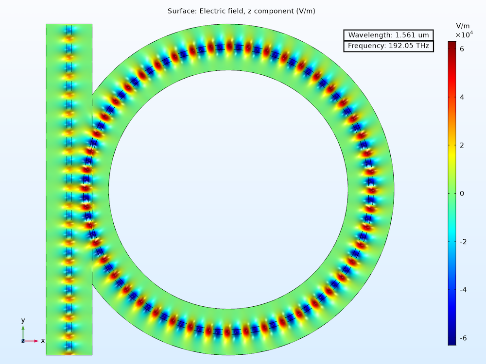 Source: Comsol
I was thinking about it a bit more and realized that a cool application for the resonator could be measuring dk / df really accurately1. This was actually inspired by the cavity resonators, since split cavity resonators exist to measure that already. Benefit of measuring with a resonator is that you can have some higher accuracy because you’re comparing in frequency spread rather than an exact wave amplitude - it’s essentially a relative measurement that is more accurate if measured resonance is actually at the right frequency.
Theory
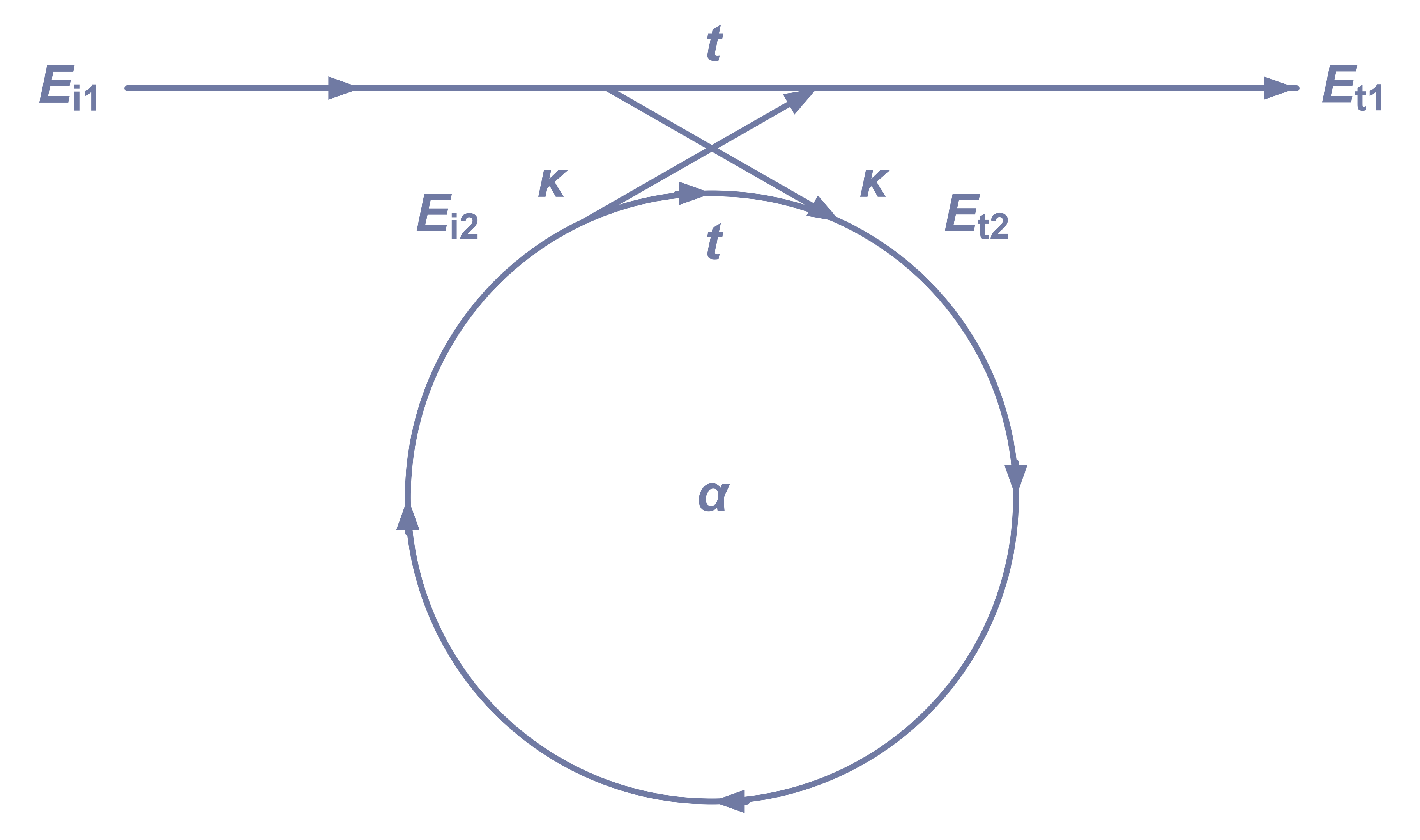
Most of this is copied from the first chapter of integrated ring resonators and follows methods from this paper for extracting loss, so I’m going to go quick here. The resonator is modeled as a coupler section (where the feed is adjacent to the ring) and a transmission line section (capturing the feed and the ring itself). The idea is that losses are modeled in the transmission lines, and the coupler is ideal. Thus we can write wave amplitudes in matrix form:
\[\vec{E_f}=\begin{pmatrix} t & \kappa \\ \kappa & t \end{pmatrix}\vec{E_i}\]Where $t, \kappa$ are transmission and coupling wave coefficients. Because the coupler is modeled as ideal, it is lossless and the matrix is both unitary and reciprocal2. From unitary condition ($S^{^{\dagger}}S=1$):
\[t\kappa^*+t^*\kappa=0\]Which implies that $t, \kappa$ are out of phase by $j$. That is, whenever the wave couples from the feed to the ring, it incurs a phase offset of $j$. If you now model the lines as ${} \alpha e^{-jk^{\prime}z} {}$ where $\alpha=e^{-k^{\prime\prime}}$ is the attenuation, you can write out that power transmission is given by
\[T^2=\frac{\alpha^2+|t|^2-2\alpha|t|\cos(\theta+\phi_{t})}{1+\alpha^2|t|^2-2\alpha|t|\cos(\theta+\phi_{t})}\]Where $ t $ is transmission factor (through the coupler part of the ring) and $\theta$ is phase propagation of the wave through the coupler, and is proportional to $f$. Plotted against frequency we can see how the resonator works:
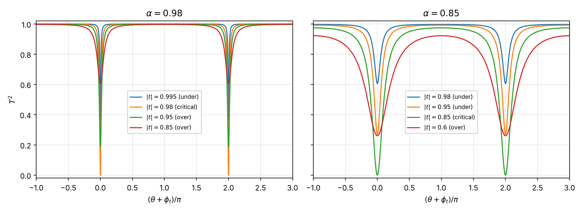
Whenever the wave circulating in the ring is coherent (in phase with factor $ 2\pi m $ ) with the input wave, there is perfect attuation of the wave - two trips between the feed and ring result in $ 2j $ phase accumulation, so the wave in the ring actively blocks the input feed. Result is that you get very sharp peaks of attenuation, super cool!
From here it is easy to measure dk because that defines the point of resonance. Resonance condition is $k^{\prime}_{z}z = 2\pi m$ (z along path length). Expanding:
\[k'_{z}z = \frac{\omega}{c}=\frac{(2\pi)^2 f\sqrt{ \epsilon_{eff} }}{c}r\]Then we can back out dk from $\epsilon_{eff}$ with closed form model like hammerstad-jensen for microstrip.
Loss is a little more tricky because layer stackups typically aren’t symmetrical about a single copper plane. It would be nice to have L2 be encased in same ply prepreg on both sides, but none of the vendors I use have a stackup like that (uncommon for low layer count boards, I think). As a result, I think it’s actually easiest to measure this in microstrip since you can then assume air is lossless and there are good models for that (again, like hammerstad-jensen).
To measure loss, we can use methods from the optica paper. The idea is that you work in the finnesse and extinction ratios:
\[\begin{aligned} F = \frac{\Delta \lambda_{FSR}}{\Delta \lambda_{FWHM}} \\ E = \frac{T_{max}}{T_{min}} \end{aligned}\]Keeping their wavelength notation here, but it’s a clear proxy for $f$. Both $F, E$ can be read directly off measured data. We can write these out explicitly in terms of $\alpha, t$ by using the transmission formula:
\[\begin{aligned} E = \left[\frac{(\alpha+t)\,(1-\alpha t)}{(\alpha-t)\,(1+\alpha t)}\right]^{2} \\ \cos\left(\pi/F\right) = \frac{2\alpha t}{1+\alpha^{2}t^{2}} \end{aligned}\]And we can then write $\alpha, t$ in terms of $A, B$:
\[\begin{aligned} A &= \frac{\cos\left(\pi/F\right)}{1+\sin\left(\pi/F\right)} \\ B &= 1-\left[\frac{1-\cos\left(\pi/F\right)}{1+\cos\left(\pi/F\right)}\right]\frac{1}{E} \\ (\alpha, t) &= \left(\frac{A}{B}\right)^{1/2} \pm \left(\frac{A}{B}-A\right)^{1/2} \end{aligned}\]We are interested in $\alpha$, and this can easily be determined using Pozar’s equations (section 3.8) for lossy quasi-TEM line:
\[\begin{aligned} \alpha_d &= \frac{k_0 \epsilon_r (\epsilon_e - 1) \tan\delta}{2\sqrt{\epsilon_e}\,(\epsilon_r - 1)} \ \text{Np/m} \\ \alpha_c &= \frac{\sqrt{ \omega \mu_{0} }}{\sqrt{ 2\sigma }Z_0 W} \ \text{Np/m} \end{aligned}\]Isolating $\alpha_{d}$ requires a good model of conductor loss, which you can get either by measuring a straight line, or by assuming properties of copper / gold with a good roughness model. You can get roughness on an SEM with 3d reconstruction features. Then it’s easy to get $\tan \delta$, the df, out.
I’m building the resonators to actually test this now. Hopefully will be able get some good measurements soon!