I’m working my way up to designing a 4x4 element phased array antenna at 5.8GHz. The idea is that two of them will be able to communicate with each other while one of them is moving, which means that they both need to be able to beamsteer. Just to get a better idea of how beamsteering works, I simulated a few simple beamforming methods..

Phased Array background

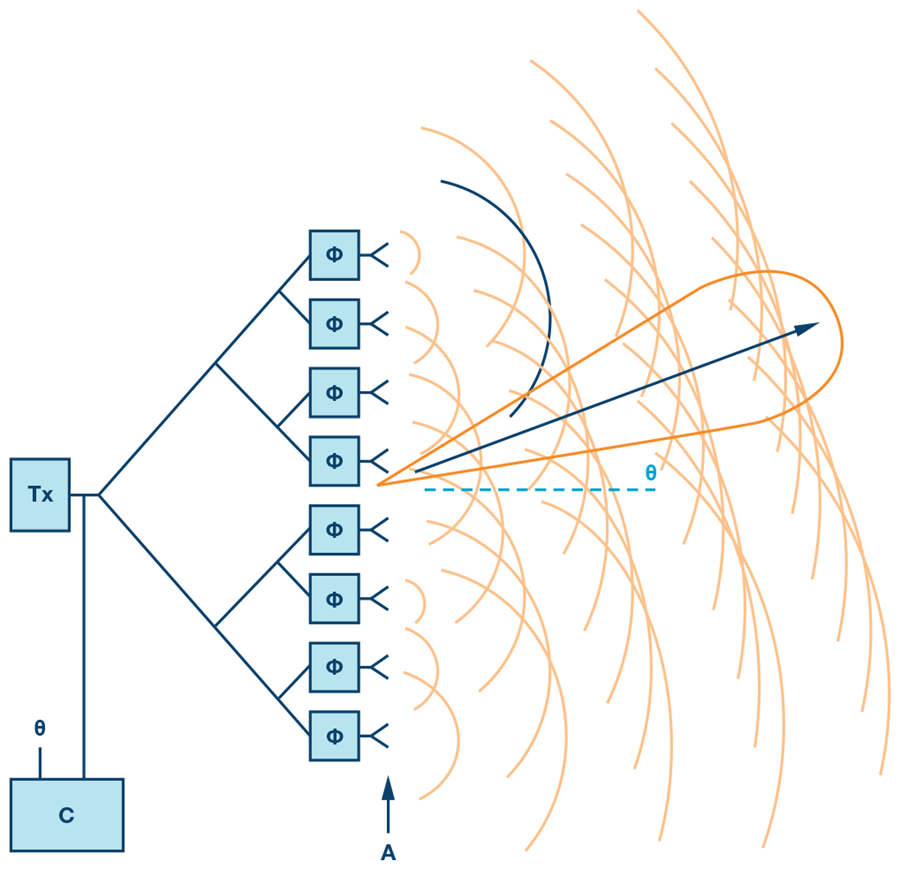
The basic idea of a phased array is pretty straightforward - it’s an array of antennas, where each has a different, electrically-controlled phase to allow for dynamic movement of the total output radiation. The most basic form of a phased array is a uniform (equally spaced and identical elements) linear (in a line) array. Then if we assume that each antenna element radiates in a nice circular shape and we phase shift teh radiation by a bit for each element in the beam, they’ll form a uniform, flat wavefront that in steered in a direction:

Now let’s put some math to this - in this post I’m going to stick to these uniform linear arrays located on the $\hat{x}$ axis and $\phi$ will be the angle off that axis (the azimuthal, by convention). To keep things simple, I’m also going to assume that each element is a hertzian dipole. Then the total radiation in the far field (near-field radiation either dies out or is stored close to the source) is given by

\[\begin{align} \overline{E}_{ff}=\sum_{i=0}^{N-1}\widehat{\theta} \frac{j\eta_{0}kI_{i}d_{i}}{4\pi r_{i}}e^{-jkr_{i}}\sin(\theta_{i}) \end{align}\]

When the target is sufficiently far away from the antenna, the Fraunhofer farfield approximation becomes valid:

\[\begin{align} r_{i}\approx r- \widehat{r} \cdot \overrightarrow{a}_{i} \end{align}\]

And then you can separate the far field into two components - the coefficient out front that captures the radiation of a single element, known as the element factor, and the sum that captures the geometry of the array, known as the array factor:

\[\begin{align} \overline{E}_{ff}=\widehat{\theta} \frac{j\eta_{0}kI_{i}d_{i}}{4\pi r_{i}}e^{-jkr}\sin(\theta)\sum_{i=0}^{N-1}w_{i}e^{jk\widehat{r}\overrightarrow{a}_{i}} \end{align}\]

The array factor is the important part since it captures the phase between array elements, which is a function of both the commanded phase ($w_i$) and the phase due to geometry and the target angle (the exponential term). $\hat{r}$ is the unit vector in the direction of the target, and $\vec{a}$ is the vector pointing from the center element of the array (or any reference element) to the others.

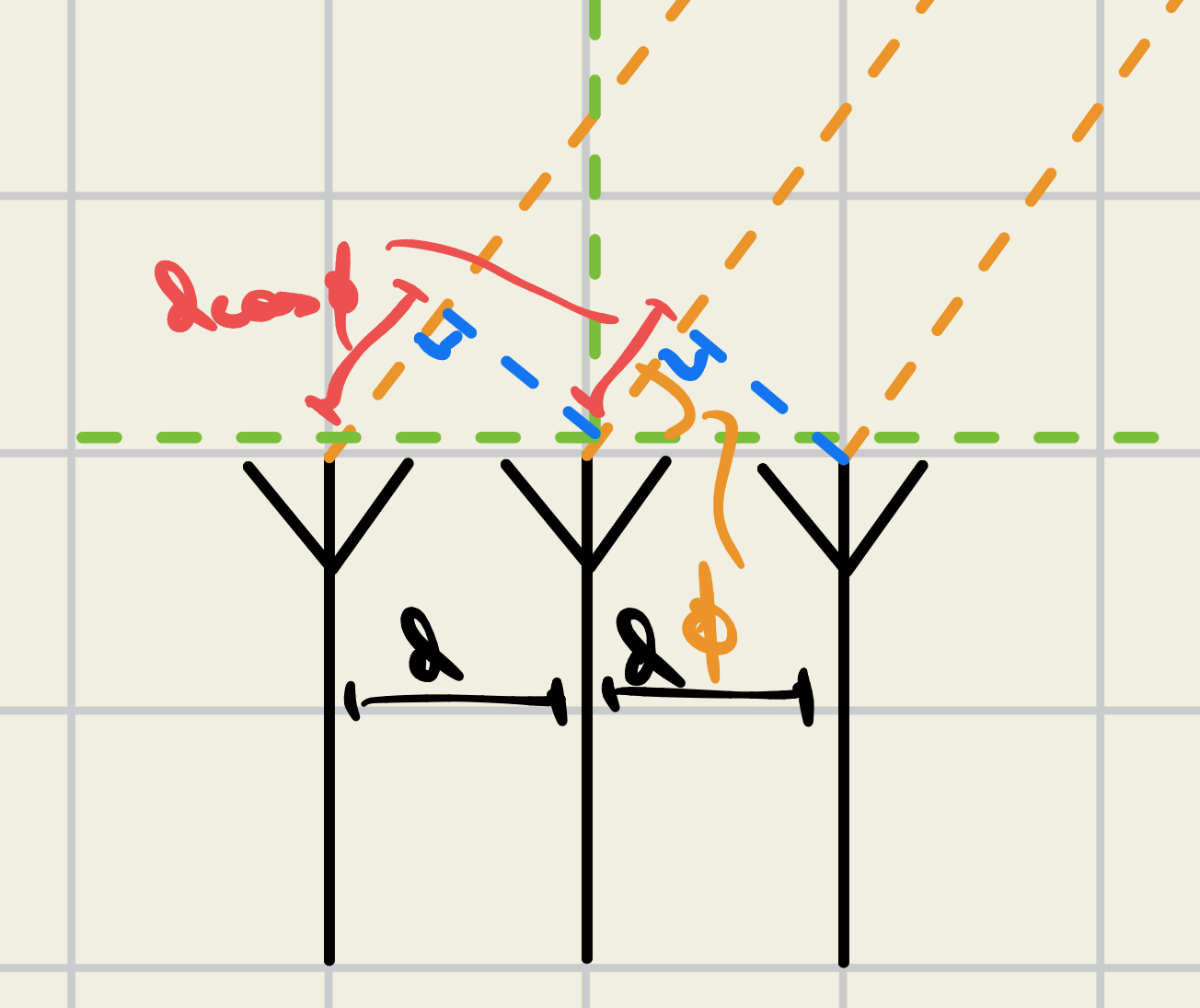
If we stay in the xy plane ($\theta = \frac{\pi}{2}$), then this is simply a cosine term

\[\begin{align} \widehat{r}\cdot \overrightarrow{a}_i = id\cos(\phi) \end{align}\]

… which will exist in the summation. $i$ accounts for increased phase as you traverse across the array. To beamsteer (radiate in different directions) all you need to do is change $\phi$. This animation shows beamsteering from $\phi =0$ to $\phi = \pi$ radians by the two elements located on the red circles.

One quick thing to point out: beamforming for receive and transmit is identical. Steering an array to radiate in direction $\phi$ requires the same weights that the array would need to receive at angle $\phi$.

Adaptive Beamforming

For my application, I’m both interested in transmitting and receiving from unknown directions since both phased arrays will communicate back and forth, they both need to know where the other is. This is where adaptive beamforming comes in - constantly updating the angle being steered at to maximize signal power from the direction of interest. The methods I’m going to go over are conventional, bartlett, and MVDR beamforming. These are pretty efficient and accurate for no more than a few beams (including sidelobes). The two other algorithms used are ESPRIT and MUSIC, which are both cool but are probably too compute intensive for me to implement on my own array. Not focusing on them now.

Noise model

Define the steering vector $\vec{s}=[e^{-jkd\cos(\phi)} \quad e^{-2jkd\cos(\phi)}\dots \quad e^{-Njkd\cos(\phi)}]^T$ as the phase lag perceived by each element in the linear array based on the angle of the incoming signal from the azimuthal $\phi$. We model the set of incoming signals as:

\[Y_{N\times T}=\vec{s}_{N}(\theta)\vec{x}_{T}^T+W_{N\times T}\]

Where $\vec{x}$ describes the data sent over some $T$ samples with $W_{ij}\sim N(\mu,\sigma^2)$ (for simplicity, notes assume $N(\mu, \sigma^2)\sim \Phi$. To model multiple angles of attack, we modify $\vec{s},\vec{x}$ to matrices to allow convenient superposition of unique $\phi$ so:

\[Y_{N\times T}=S_{N\times \phi}(\theta)X_{\phi \times T}+W_{N\times T}\]

Where for ${} M$ directions $\phi$:

\[S_{N\times M}=\begin{pmatrix} \vec{s}_{N, \phi_{1}} & \vec{s}_{N, \phi_{2}} & \dots \vec{s}_{N,\phi_{M}} \end{pmatrix}_{N\times M}\]

and

\[X_{M\times T}=\begin{pmatrix} x^T \\ x^T \\ \dots \\ \end{pmatrix}_{M\times T}\]

Code

def random_complex_sines(f, samples, aoas):
  # Returns matrix: aoas x samples
  output = []
  for _ in range(aoas):
    random_f = f * np.random.uniform(low=-0.5, high=0.5)
    signal = np.random.normal(1, 0.1) * np.sin(2 * np.pi * (random_f * samples + np.random.rand()))
    output.append(signal)
  return np.array(output)

def noisy_signals(directions, signals, variance):
  # Steer - Nxaoas
  steer = np.exp(1j* 2*np.pi*d * np.outer(np.arange(N), np.cos(directions)))

  # Random NxT noise
  w = (np.random.randn(N, len(signals[0])) + 1j*np.random.randn(N, len(signals[0]))) * np.sqrt(variance/2)
  receive = steer @ signals + w
  return receive

Signal amplitude is normal with with mean $\mu=1, \sigma^2=0.1$ to make the sim a little more interesting; for all intensive purposes this is 1 for SNR computation.

Power-Variance Relationship

Mathematically, variance is constructed the same as power (ignoring scaling constants / units). This should be pretty obvious from their formulas:

\[\begin{align} P &= \frac{1}{N} \sum_{n=0}^{N-1} x[n]^2 \\ x_{\mathrm{RMS}} &= \sqrt{\frac{1}{N} \sum_{n=0}^{N-1} x[n]^2} \\ \sigma_x^2 &= \frac{1}{N} \sum_{n=0}^{N-1} \left(x[n] - \mu_x \right)^2 \end{align}\]

This is a neat duality and is why you can combine probabilistic quanities (noise power) with physical ones (real power). The two assumptions this makes though is

1. Processes are wide sense stationary (mean and variance constant across time)¹
2. Processes are ergodic - time average of a single process is the ensemble average; this justifies the notion that a single sample can represent all possible samples, hence polling it many times will yield the ensemble itself.

These two requirements allow the probabilistic methods below.

Conventional beamforming

Very simple - performs a shift on all incoming signals for a given angle of attack $\theta$, then adds them up to get an idea of how correlated they are (i.e. computes cross correlation).

Assuming that $W_{ij}$ is small relative to the input signal (the SNR is high), we just shift $\vec{y}$ by a “test” angle $\theta_{t}$ using the hermitian (conjugate transpose) of $\vec{s}$:

\[\vec{p}_{T}=\frac{1}{N}\vec{s}^HY\]

Where the conjugate is useful because it flips the phase lag. This returns a signal of size $T$. We can take compute the variance (rms power squared) to determine if the test angle is a probable angle of attack; power will be high when the signals add constructively through the test angle vector $\vec{s}$.

Then you end up with a single signal representing the normalized ‘average’ of the $N$ incident signals; compute the variance of each as you sweep over $\theta$, and select the one with highest variance (highest since the signals will add constructively when they are aligned properly).

def delay_sum(test_phi, noisy_signal):
  test_steer = np.exp(1j* 2*np.pi*d * np.linspace(0, N-1, N) * np.cos(test_phi))[:, np.newaxis]
  reconstructed = 1/N * test_steer.conj().T @ noisy_signal
  signal_power = np.var(reconstructed)
  return signal_power

Not robust because it requires high SNR.

Bartlett Beamforming

Bartlett beamforming is identical to conventional beamforming, so I’m not sure why it has a different name. What is helpful about it is that it formulates the problem in the frequency / probabilistic domain, which gives useful insight.

The ideal beamformer would yield an ideal output signal:

\[p(\theta_{t})=\frac{1}{N}\vec{s}^H\cdot Y\]

Now we compute the variance directly:

\[\begin{align} P&=\frac{1}{N^2}\mathbf{E}[(\vec{s}^H\cdot Y)^2] \\ &=\frac{1}{N^2}\mathbf{E}[(\vec{s}^H\cdot Y)(Y^H\vec{s})] \\ &=\frac{1}{N^2}\vec{s}^H\mathbf{E}[YY^H]\vec{s} \\ &=\frac{1}{N^2}\vec{s}^HR_{YY}\vec{s} \end{align}\]

Where $R_{YY}$ is the spatial autocovariance matrix of $Y$. Keep expanding the expression:

\[\begin{align} P&=\frac{1}{N^2}\vec{s}^H(\mathbf{E}[(SX+W)(SX+W)^H])\vec{s} \\ &=\frac{1}{N^2}\vec{s}^H\left( \vec{s}_{\phi} \left( \sum_{i\in \{1\dots T\}}|x_{i}|^2 \right) s^H_{\phi} +TI_{N\times N}\right)\vec{s} \\ &=\frac{1}{N^2}\left(\bar{s}\left(\sum_{i\in \{1\dots T\}}|x_{i}|^2\right)\bar{s}+TN\right) \\ &=\frac{\bar{s}^2}{N^2}\sum_{i \in \{1\dots T\}}|x_{i}|^2+\frac{T}{N} \\ &=\frac{\bar{s}^2}{N^2}P_{sig}+P_{noise} \end{align}\]

Note that in the general case where there are multiple steering angles $\phi$, $\vec{s}$ is the vector of scalar sums of many complex exponentials representing shifts from multiple incident phase angles $\phi$ on a single element denoted $\vec{s_{\phi}}$. For a $\vec{s}$ that matches the steer of one of these $\phi$, we see one angle go to unity, but will still have many complex exponential shifts for those $\phi_{i}\neq \phi_{test}$. This is interesting because $\phi_{test}\propto d$, so the resulting phases are both functions of $d$ (array geometry) and the various $\phi_{i}$ (source angles of arrival). This arbitrary complex scaling is represented by $\bar{s}$². When the test angle matches the steering angle, $\bar{s}^2=N^2 + C$, where C is a messy polynomial from other angles of attack.

This final expression is what you would expect; power level for ‘correct’ steering angle (restricting the scope here to a single $\phi$) is the sum of signal power and noise power. The noise power here matches expected noise power of the sample mean across all time (if we took $W_{ij}\sim N(\mu \neq 0, \sigma^2\neq 0)$ we would see a noise power of $\frac{\sigma^2}{N}$, as expected).

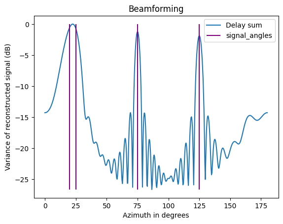
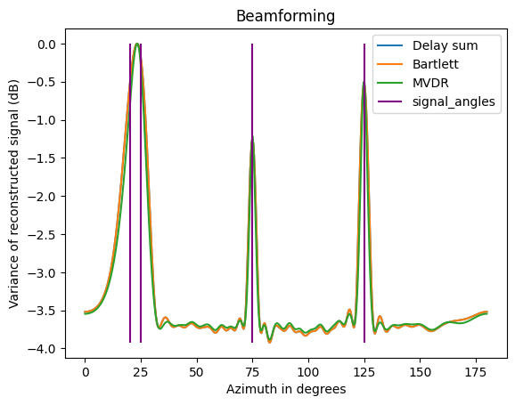
I simulated the output power from each algorithm. Array model is with 30 elements and half wave spacing. There are four incident angles - 20, 25, 75, 125 degrees.

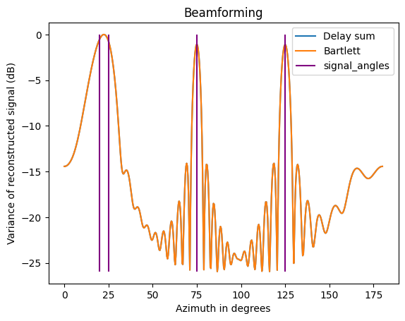
Two clear observations are that

1. Both the bartlett and delay sum are on top of each other, they are identical
2. Lots of noise in the stopband, which is really just the sidelobes. The algorithms maximize signal power, resulting in a condition where they are steering ‘into’ a sidelobe.

def bartlett(test_phi, Ryy):
  test_steer = np.exp(1j* 2*np.pi*d * np.linspace(0, N-1, N) * np.cos(test_phi))[:, np.newaxis]
  signal_power = 1/N**2 * test_steer.conj().T @ Ryy @ test_steer
  return signal_power.item() # need to use item to pop number out of 1x1

Capon (MVDR) beamformer

The MVDR (minimum variance distortionless response) beamformer uses the same construction as the Bartlett in the frequency domain but optimizes over the test steering matrix $\vec{s}$ to minimize noise power, subject to the condition that it actually steers in the right direction. This allows sidelobe rejection:

\[\begin{aligned} \min \quad & \vec{s}^H R_v \vec{s} \\ \text{subject to} \quad & \vec{s}^H a(\phi_{d}) = 1 \end{aligned}\]

Where $R_{v}$ is the noise covariance matrix. But we have no real knowledge of $R_{v}$, and instead use $R_{YY}$ as a proxy:

\[\begin{aligned} \min \quad & \vec{s}^H R_{YY} \vec{s} \\ \text{subject to} \quad & \vec{s}^H a(\phi_{d}) = 1 \end{aligned}\]

The constraint forces $\vec{s}$ to be a proper steering vector (normalizes against an angle $\phi$). This can be accomplished with a variety of $\vec{s}$; the objective forces $\vec{s}$ to focus on the lowest power solution, thereby minimizing sidelobes. Using lagrange multipliers, you can solve the optimization problem, yielding

\[\vec{s}= \frac{R_{y}^{-1}a(\theta)}{a(\theta)^HR_{y}^{-1}a(\theta)}\]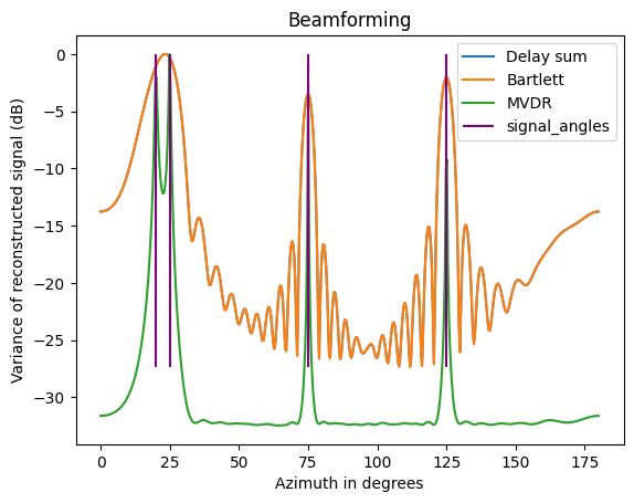

Computing the spatial autocovariance matrix:

Ryy = (noisy_reception @ noisy_reception.conj().T) / noisy_reception.shape[1]
delta = 1e-6 * np.trace(Ryy)/N
Ryy_loaded = Ryy + delta*np.eye(N)
Ryy_inv = np.linalg.inv(Ryy_loaded)

The reason for Ryy_loaded is that $R_{YY}$ can sometimes be ill-conditioned, causing numerical errors during the matrix inversion. I added this just in case but never noticed a difference in sim.

Implementation:

def mvdr(test_phi, Ryy, Ryy_inv):
  test_steer = np.exp(1j* 2*np.pi*d * np.linspace(0, N-1, N) * np.cos(test_phi))[:, np.newaxis]
  weights = Ryy_inv @ test_steer / (test_steer.conj().T @ Ryy_inv @ test_steer).item()
  signal_power = weights.conj().T @ Ryy @ weights
  return signal_power.item() # need to use item to pop number out of 1x1

Observations

Grating lobe rejection

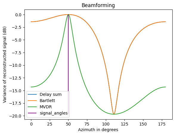
None of the above algorithms should be able to compensate for grating lobes. This is a spatial aliasing that none can reject. We can see this clearly with one incident angle $\theta=0$ and element spacing set to full wave:

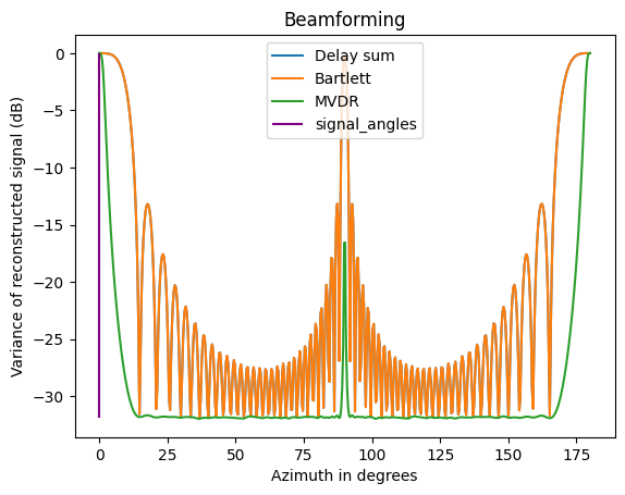
There is a big grating lobe in the middle.

MVDR convergence with poor snr

For very low SNR (specifically, high additive noise power relative to sidelobe noise power) MVDR should converge on all the sidelobes; extreme example here with SNR of -20db:

Received signals	Recovered Power

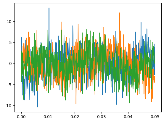Effectiveness with few elements

With fewer elements, there are fewer sidelobes but they are larger. MVDR is much better at handling this case, as expected; this is with two elements:

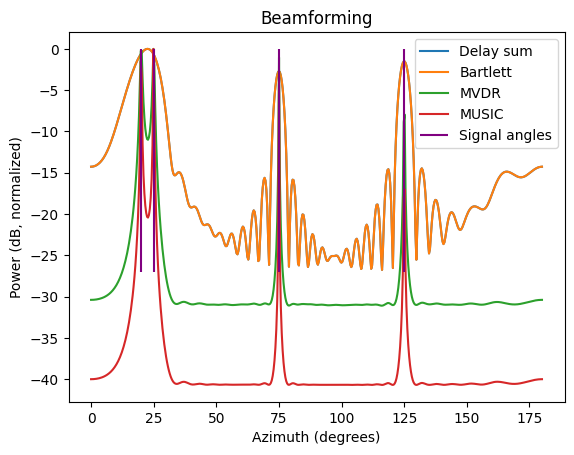
MUSIC

MUSIC doesn’t really rely on probabilistic methods. I think wikipedia gives a good explanation, but here’s a rough summary. Instead of doing an optimization / computation over power, it exploits the fact that $R_{YY}$ is hermitian, so columns are orthogonal to each other and it is diagonalizable. Music performs an eigendecomposition on $R_{YY}$ and reorders the eigenvectors / values by the size of the eigenvalues, thereby separating $R_{YY}$ into a signal subspace $U_{s}$ and a noise subspace $U_{n}$. A test steering vector $\vec{e}$ is necessarily in the signal subspace, but is orthogonal to the noise subspace. Thus, define a norm to quantify how orthogonal $\vec{e}(\phi_{test})$ is to the noise subspace:

\[d^2=\mid U_{N}^H\vec{e}(\phi_{test})\mid^2=\vec{e}^HU_{N}U_{N}^H\vec{e}\]

Intuitively, the steering angle that matches a target angle $\phi$ is exactly orthogonal to the noise subspace by virtue of being in $U_{s}$ itself, thereby $d^2$ small. By inverting we get peaks that clearly show detected signal eigenvalues (frequencies $\sim\phi$).

To order / separate the eigendecomposition:

eigenvalues, eigenvectors = np.linalg.eigh(Ryy)
num_sources = len(aoas)
noise_eigenvecs = eigenvectors[:, :N - num_sources]

music implementation:

def music(test_phi, noise_eigenvecs):
  test_steer = np.exp(1j* 2*np.pi*d * np.linspace(0, N-1, N) * np.cos(test_phi))[:, np.newaxis]
  proj = noise_eigenvecs @ noise_eigenvecs.conj().T
  power = 1 / (test_steer.conj().T @ proj @ test_steer).real
  return power.item()

MUSIC signal separation

One of the advantages of MUSIC is that it separates closely spaced signals extremely well:

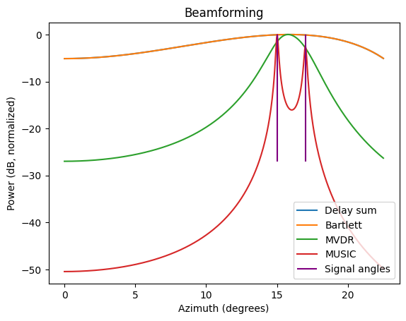
It appears to perform better than mvdr in general, with lower stopband and sharper SNR in its frequency selection. Only caveat is computational speed, since eigendecomposition typically takes longer than matrix inversion in practice (though both are $\Theta(n^3)$, so difference might be small if $R_{YY}$ is computed for long timescale).

(Cover image courtsey of Analog Devices)

1. Intuitively it feels strict sense stationary would be true too, though maybe high order terms are constantly changing to this is unnecessarily strong ↩

2. Let’s focus a bit more on the construction of this. Expanding $\vec{s}_{\phi}$:

   $$ \begin{align} \vec{s}_{\phi}=\begin{pmatrix} e^{jk(1)d}\sum_{i}e^{\cos(\phi_{i})} \\ e^{jk(2)d}\sum_{i}e^{\cos(\phi_{i})} \\ \dots \\ e^{jk(N)d}\sum_{i}e^{\cos(\phi_{i})} \\ \end{pmatrix} \end{align} $$

   The test angle vector $\vec{s}$ is

   $$ \begin{align} \vec{s}=\begin{pmatrix} e^{jk(1)d\cos(\phi_{test})} \\ e^{jk(2)d\cos(\phi_{test})} \\ \dots \\ e^{jk(N)d\cos(\phi_{test})} \\ \end{pmatrix} \end{align} $$

   Thus

   $$ \vec{s}^H\vec{s}_{\phi}=\sum_{n=0}^{N-1}e^{jknd(\cos(\phi_{i})-\cos(\phi_{test}))}+C $$

   Where C is some messy complex polynomial accounting for all the other $i$. Notice that when there is a single source and $\phi_{i}=\phi_{test}$ the inner product goes to $N$. ↩