Since taking electromagnetics, I’ve been looking for an RF engineering project. After reading Henrik’s blog, an FMCW radar seemed like a good one; the board hardware is all RF engineering, I can experiment with some antenna design while testing, and the final goal of the project - extracting a doppler range plot - requires some dft. Lots of fun stuff to learn!

Background

Here’s a quick rundown of FMCW radar.

The working principle is that you send out a continuous wave modulated in frequency (usually by a sawtooth, or the “chirp”) and centered around some baseband (in this case, 5.8GHz). Since the wave is continuously sent out, once it reflects on the target, propagates back towards the radar, and is received, all the radar needs to do is take the difference between the received frequency and the frequency transmitted at the same instant. That difference is related to the phase lag / propagation time to the target, and thus the distance to the target (by the speed of light). The reason a sawtooth chirp is popular is because it makes the relation between the phase lag and the frequency linear, so the processing you need to do after receiving the signal is super easy.

Generalizing this, if your beam actually hits multiple targets, you expect the superposition of multiple chirps to be received back. All you need do is perform the frequency subtraction again, but take the fourier transform before you convert to distance to digitally locate the range of each target.

For velocity, things are still pretty straightforward - you just perform the distance measurement multiple times (so that you don’t get confused, for now ignore the actual computation of the distance, and instead just imaging measuring a 2d “frequency difference plot”). Suppose a target is moving; you’ll see the frequency difference move over time — that’s related to a characteristic frequency, so you just need to take another fourier transform along the time axis of data! Now you wonder - do you need to save two copies of the data, one to do the time fourier over, and one to do the distance fourier over? Or do you need to save the whole 2d buffer? No! Notice that the distance fourier transform is decoupled from the time fourier transform, so you can do a proper 2d fourier transform: just take the fourier transform over the distance axis as time goes on, and once you’ve done that many times, take another fourier transform of those previous fourier transforms along the time axis. That makes the memory requirement for this pretty relaxed.

How do you actually implement this in hardware? I’m borrowing Henrik’s block diagram here since I’m doing exactly the same thing:

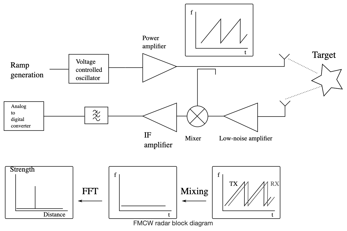
There are really only three important components: the vco, the mixer, and the adc. The vco obviously creates the RF signal - you can modulate this with a pll or a dac. The mixer performs the frequency subtraction using a reference signal split off the transmit line, and the adc is responsible for actually sampling the filtered IF to be processed.

This is going to be a multi-stage project. The first version will offload all the dft to my laptop, with data streamed from the radar over high speed usb. The sawtooth frequency chirp used in fmcw radar will be generated by the 12 bit high speed dac integrated in the on board stm32g4 ¹. The next version will have an onboard fpga and probably multiple receive channels. I’m also gonna control the vco with a pll for lower phase noise and better control over the chirp parameters - usually those chips let you chirp much faster and with arbitrary waveforms too.

Design

I picked the 5.8GHz ISM Band because I wanted to be in the GHz range for some extra design complexity, and I expect a good amount of clutter at 2.4GHz from Wifi. At the next band up, 22GHz, there are fewer available components and their prices are a bit too high for me to justify.

I didn’t really know what I was doing, so I chose what I expected were slightly ambitious design parameters so I’d have somewhere to start:

• Max Range: 100m
• BW: 100MHz
• Chirp time: 1mS
• Minimum cross section: 1m^2

The radar range and the spread of targets it can measure also depends on the antenna used. To keep things simple, I’m designing for 5.8GHz patch antennas used for drone fpv video. In the future, I’ll probably design a linear patch array to reduce the gain in the direction of the ground.

Layout

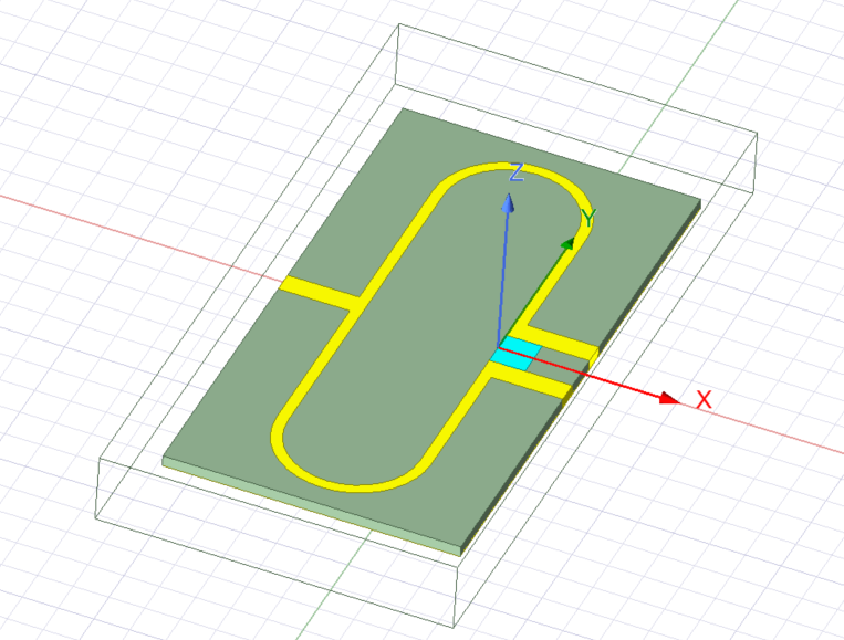
Wilkinson Power divider²

This was one of the trickiest parts of the design, mostly because I had to learn HFSS. I started by designing something that looked like a wilkinson, using the kicad transmission line calculator for trace widths. I also used terminal lumped ports.

That gave me shitty looking plot like this:

From S11 you can clearly see that the input impedance isn’t 50Z - there’s a huge reflection. I modeled microstrips independently to tune the widths in, and discovered that the kicad calculator was wayyy (like close to 50%) off of the target impedance of 50Z and 70.7Z. That led to a long, two-day rabbithole of trying to figure out what the most accurate calculator / formula / paper is, to save time next time. I came to the conclusion that the equations in Pozars are the most accurate for most stackup geometries. It seems like any formula for the impedance that is piecewise is fairly accurate, and all the others are only accurate in the correlatation between microstrip parameters and the impedance.

As a quick aside - I ran into a lot of problems with actually setting up the simulations for measuring microstrip characteristic impedance accurately, mostly because I didn’t understand the differences between lumped and wave ports. I made a little writeup on differences between the two.

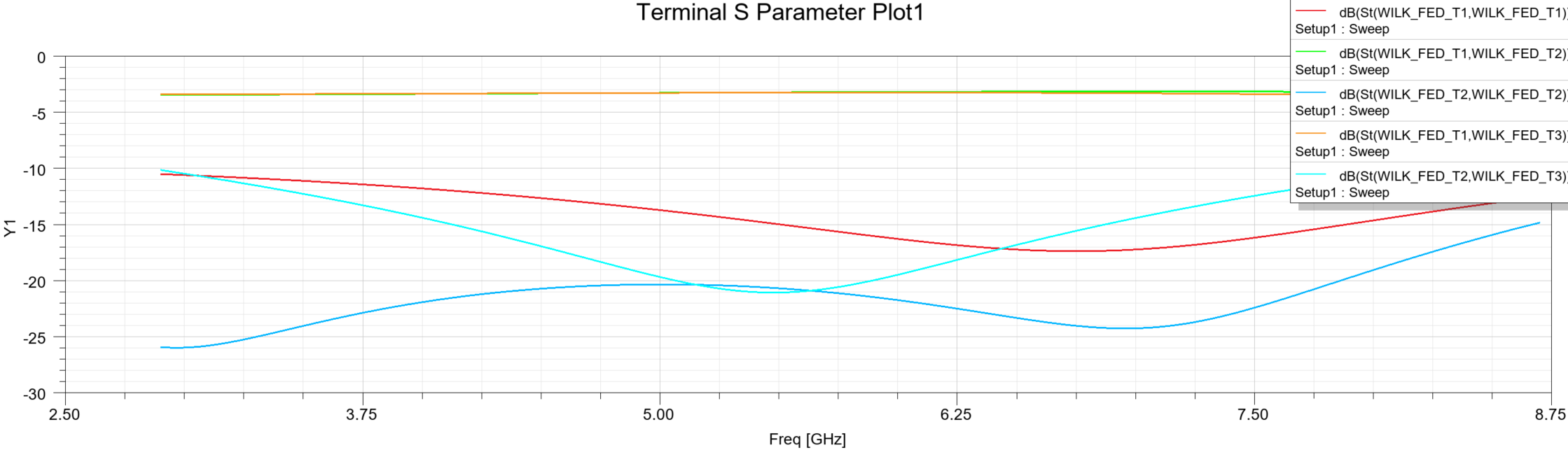
With a lot more futzing, I got something okayish that seemed accurate:

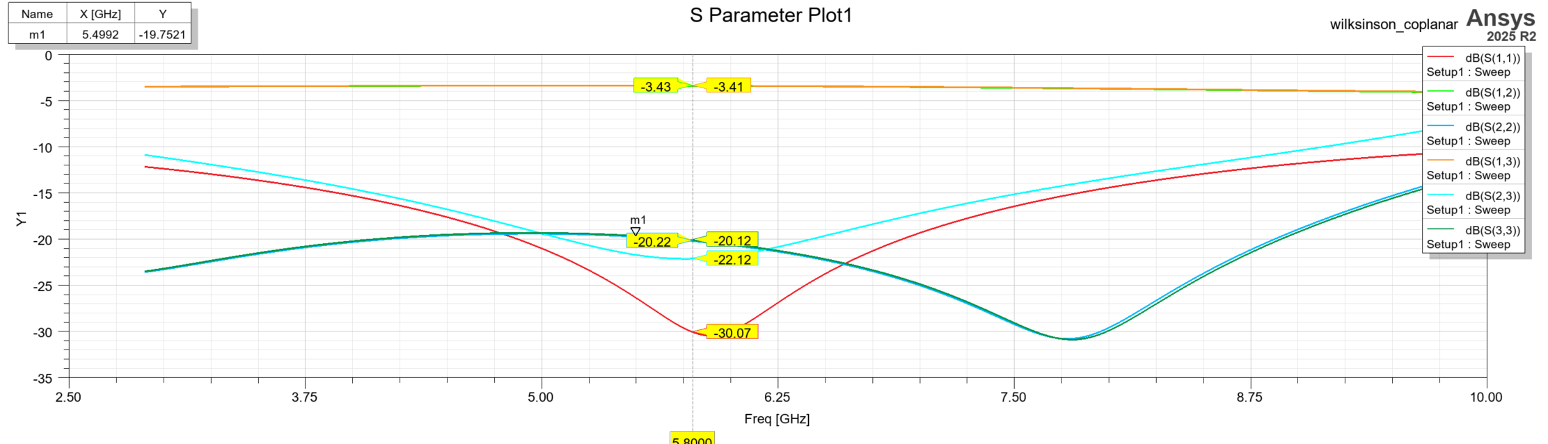
Adding a coplanar ground with fencing vias and making the resistor smaller (0201 now) improved the isolation and return loss on the other ports:

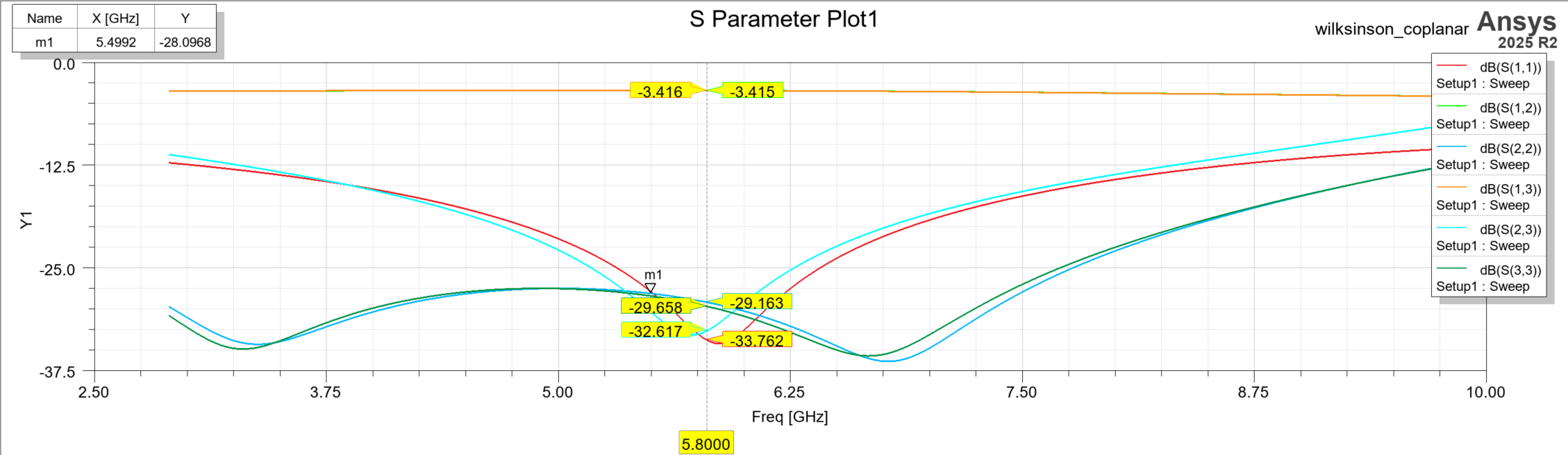
Based on some articles I read, it seemed like over -20db of isolation and return loss was considered bordlerine working, so I decided to call this design finished. I think one of the main limitations in this design is the shape of the quarterwave sections (you are forced to have a sharp corner near the resistor), so next time I might try using something more circular.

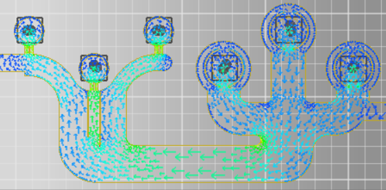
Ansys lets you view the fields, which looks really cool:

SMA transition

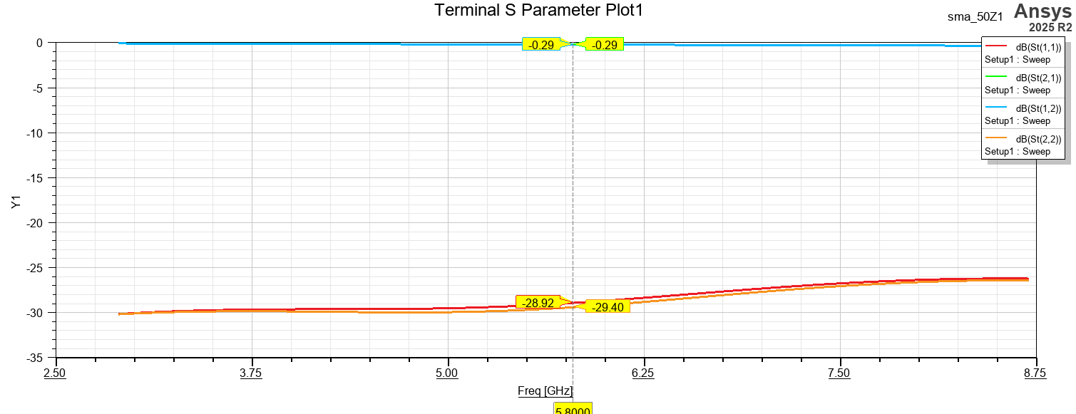
I’m using edge-mount SMA connectors, and that introduces another problem. Although the SMA needs to connect to a 50Z transmition line, the output pin of the SMA is wider than line (which is 0.37mm wide on the JLC3313 stackup). That causes the pad in the connector footprint to be wider, making it low impedance and creating a large impedance mismatch between the pad and the line. It turns out that this can be easily fixed by voiding the ground layers below the pad and tapering the connection between the pad and the line. With a bit of tuning I was able to get an ok transition:

a

1. The downside of this is that I need to manually (probably via lookup table, no feedback since the stm32 will be too slow) compensate for the VCO nonlinearity. The phase noise will probably also suck, but this shouldn’t be much of a problem since I’m not designing for great range resolution anyway. ↩

2. Why a wilkinson? Because it’s the first divider type talked about in Pozar, and the theory is really simple, so I thought it’d be easy to design. Unfortunately it turns out that theory and design complexity are not necessarily correlated. It probably would’ve been easier to make a coupled line instead (and this would’ve also made a lot more sense for the design) but, alas… ↩